For its essential importance as a resource, sustainable development of groundwater has been major research interests for many decades. Conventional characterization of aquifer and groundwater has relied on borehole data from observation well. Although borehole data provide useful information on yield and flow of groundwater, it is often difficult and sometimes costly to estimate the spatial distribution of groundwater in entire aquifer. Geophysical probing is an alternative techique that provides such information due to its capability to image subsurface structures as well as to delineate spatial distribution of hydraulic parameters. This study presents various technical information about geophysical probing to estimate main characteristics of aquifer for groundwater exploitation. Subsequently, we analyzed representative cases, in which geophysical methods were applied to identify the location of the groundwater, classify freshwater and brine, derive hydraulic constants, and monitor groundwater.

Keywords: Aquifer characterization, Groundwater, Geophysical method,Hydraulic parameter

지하수는 전세계 육지 담수의 약 30%만을 차지하지만 담수 중 69%는 빙하와 만년설로 이루어져 있기 때문에, 이용 가능한 담수 중 90% 이상을 차지하며, 평균적으로 인간이 소비하는 담수의 3분의 1을 차지하고 있기 때문에 매우 중요한 수자원이다(Shiklomanov et al., 1993). 국내 지하수 부존량은 실제 이용 가능한 수자원 총량 대비 55.3%로 미래 가치가 매우 높아(Hyun, 2014), 지하수 개발, 인공 함양, 해수 담수화와 같은 지하수 확보 노력이 증가하고 있다(Won et al., 2015; Lee et al., 2015; Jung et al., 2015). 특히 최근 들어 지표수 오염, 기후변화에 따른 계절 및 연간 강우량의 급격한 변화, 인구 증가에 의한 물 수요 증가, 경제 개발로 인한 지하수의 과도한 개발 등의 이유로 지속 가능한 지하수 개발을 위한 연구가 많이 수행되고 있다(e.g., Kadri et al., 2010; Chung et al., 2015; Lee et al., 2015; Jung et al., 2015; Gopinath et al., 2019; Azhar et al., 2019).
이러한 지하수에 대한 탐사는 식수 취수, 농업의 관개(Fitts, 2002), 환경 연구와 오염 토양 조사(Weiss et al., 2008) 및 수문학에서의 수리상수(hydraulic constant) (혹은 매개변수(parameter)) 추정과 같은 목적을 위해 수행되었다. 최근에는 CO₂ 지중저장 부지 특성화(Romanak et al., 2012), 방사능 폐기물 처리장 부지 특성화(Levchuk et al., 2012)와 같은 다양한 분야에서도 지하수의 분포와 흐름 등이 중요하여 연구가 진행되고 있다(Gloaguen et al., 2001).
국내에서 지하수 탐사는 일반적으로 대수층 평가 및 지하수를 조사하기 위해서 유역별로 나누어 관측공을 설치하여 조사한다(Lee et al., 2020). 관측공 자료를 이용하는 경우 지하수위뿐만 아니라 수리상수도 측정하여야 대수층의 개념모델(conceptual model)을 구축할 수 있다(Bhatt, 1993; Niwas et al., 2011; Frind and Molson, 2018; Ahn and Park, 2015). 시추공 조사를 기반으로 취득한 수리지질학적 매개변수들을 광범위한 공간에 걸쳐 특성화하고 모니터링하는 것은 수문학에서 가장 큰 과제다(Todd and Mays, 2004; Slater and Binley, 2021).
시추공 기반 조사는 한 지점에서의 유체 흐름에 대한 우수한 정보를 제공하지만, 이질적인 지하매질에서 단일 측정값을 더 큰 범위의 값으로 추정하는 것은 어려울 뿐만 아니라 이를 해결하기 위해 추가적으로 시추공을 설치할 경우 비용도 많이 든다는 단점이 있다(Fagerlund et al., 2003; Sattar et al., 2014). 기존에 수문학 분야에서 대수층을 3차원(3D) 영상화할 때 시추공 자료를 공간 보간(spatial interpolation)과 같은 지구통계학적 방법을 사용하지만(Gunnink et al., 2021; Chakma et al., 2022), 단순한 공간보간 방법은 물리적인 의미 없이 광활화(smoothing) 된다는 단점이 있다(Yao et al., 2014).
물리탐사(geophysical survey)는 비파괴적 방법으로 비교적 짧은 시간 동안 광범위한 지역의 내부 정보를 얻을 수 있는 방법으로 수리지질조사(Binley et al., 2015) 뿐만 아니라 산사태 지역 모니터링(Chambers et al., 2013), 유류오염 탐사(Cardarelli et al., 2009; Castelluccio et al., 2018), 지반침하 조사(Cueto et al., 2018), 광물 탐사(Fallon et al., 1997)와 같은 다양한 분야에서 적용되고 있다. 물리탐사 자료의 2차원 및 3차원 영상화를 수행하면 지하수 분포 및 흐름에 대한 정보를 얻을 수 있기 때문에(Hubbard et al., 2001; Dawoud et al., 2009), 대수층 평가를 위한 퇴적암 대수층 특성화(Dickson et al., 2014; Binley et al., 2016), 수리상수 도출(Massoud et al., 2010; Dai et al., 2010), 그리고 연안에서의 담수와 해수 구분(Fitterman et al., 2014; Graham et al., 2018)과 같은 연구도 물리탐사에 기초하여 진행되고 있다.
국내에서는 충적층 특성 평가(Won et al., 2013), 균열 암반 대수층 특성화(Cho et al., 2000; Song et al., 2002)에 대한 연구가 수행되고 있으며, 대수층 평가를 위한 방법으로 주로 전기비저항 탐사를 가장 많이 활용한다(Choi et al., 2000). 그러나 지하매질이 매우 복잡하거나 점토가 존재하는 경우에는, 등가성(equivalence)의 문제로 인하여 전기비저항 탐사만 수행하여 대수층을 평가하는 것은 한계가 있다(Kim et al., 1997). 이를 보완하기 위해 다른 물리탐사 기법이나 관측정 자료를 함께 적용하기도 한다(Olorunfemi et al., 2020; Bodin et al., 2021; Gonzalez et al., 2021).
이 논문에서는 먼저 대수층의 종류별 특성에 대해 알아보고, 대수층에서 파악할 수 있는 물성 및 현상과 이로 인한 물리탐사를 이용한 대수층 특성화 방법, 대수층 특성화 와 현장 적용성과 방법에 대해 기술하였다. 이후 실제 지하수 탐사를 수행한 물리탐사 사례들을 탐사 목적에 따라 분석하였다.

2.1. 대수층 특성
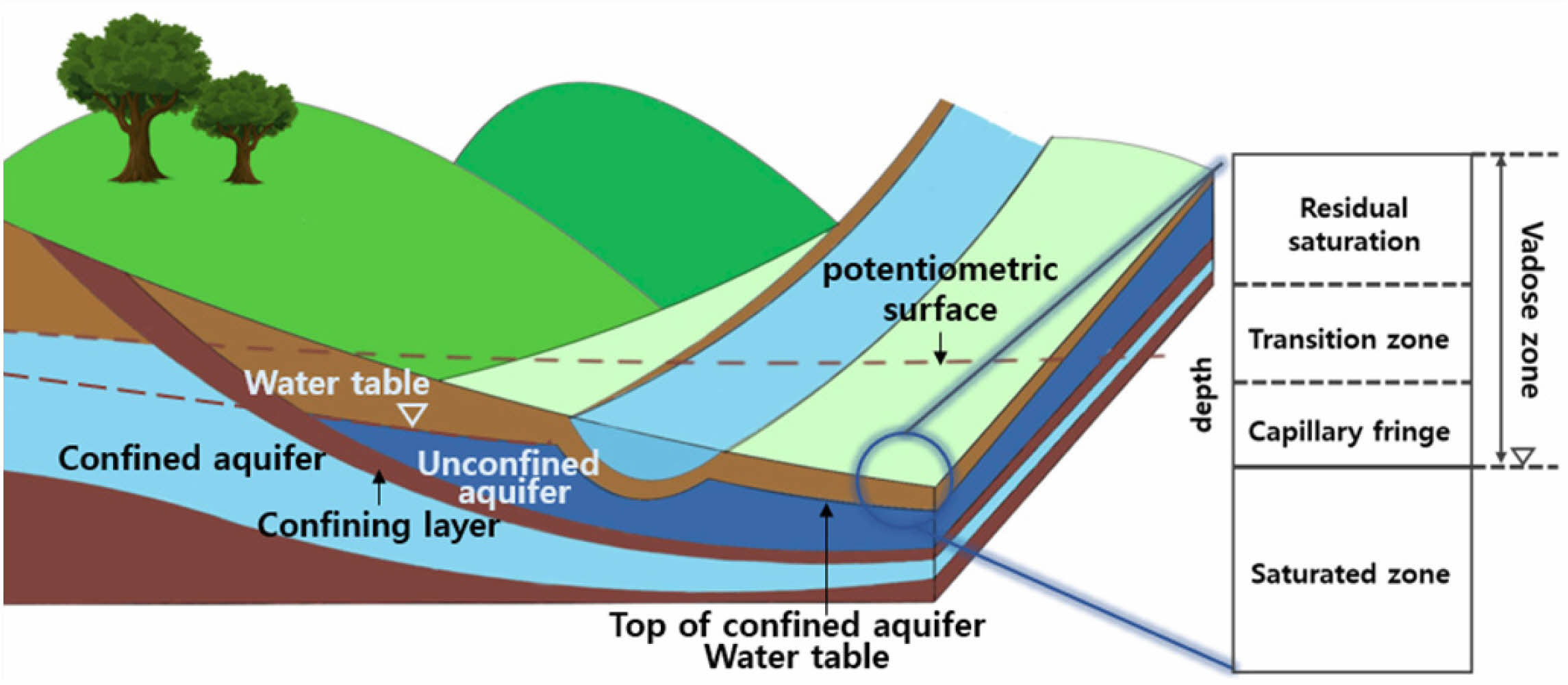
대수층은 크게, 지하수에 의해서 토양 내부 공극이 완전히 지하수로 채워져 있는 포화대와, 부분적으로 물로 포화된 공극이 주로 공기로 채워져 불포화대로 나눌 수 있다(Fig. 1). 포화대와 불포화대의 경계면인 지하수면 위쪽에 위치하는 불포화대는, 잔류포화대(residual saturation), 모관대(capillary fringe), 모관대와 잔류 포화대 사이의 중간대(transition zone)로 구분할 수 있다(Kelly et al., 1993). 지질학적 환경에 따라서 대수층은, 피압대수층(confined aquifer), 자유면대수층(unconfined aquifer), 주수대수층(perched aquifer)으로 구분할 수 있다(Batu, 1998) (Fig. 1). 이러한 대수층은 지질학적 체계를 구성하는 퇴적물이나 암석의 광물 조성, 입자 크기, 압력 등을 포함한 물리적 구조에 따라서도 나눌 수 있는데, 지하매질을 구성하는 암석의 특성에 따라서는 크게 퇴적층 대수층, 충적층 대수층, 암반 대수층 등으로 분류할 수 있다(Todd and Mays, 2004). 국내 대수층은 주로 충적층 대수층이나 암반 대수층이 주를 이루며(Lee et al., 2007), 제주도와 같이 독특하게 현무암 지대에 발달되어 있는 경우도 있다(Hamm, 2005). 여기에서는 먼저 이들 대수층의 특징을 알아본 뒤, 연안에 위치한 대수층과 점토질을 포함한 대수층의 특성에 대해서도 살펴본다.

- 퇴적층 대수층(sedimentary aquifer)
퇴적층 대수층으로 크게 사암, 탄산염암, 석탄(coal) 대수층 등이 있다. 사암은 전세계 퇴적암의 약 25%를 차지하는 세립질 입자를 가진 암석으로 입자 사이의 간격은 매우 작지만 전체적인 공극률이 커 많은 양의 물을 함유할 수 있기 때문에, 많은 나라에서 사암 지층은 많은 양의 물이 존재하는 대수층을 형성하고 있다(Freeze et al., 1979). 탄산암이 육지에 노출되어 있는 곳에서는 카르스트 지형의 대수층이 생성되는(Freeze et al., 1979) 반면, 셰일과 같은 불투수성(impermeable) 퇴적암은 물을 저장하고 있거나 물의 유동을 느리게 하는 반대수층으로 작용하여 즉 물의 흐름을 막아 주변에 대수층이 형성될 수 있는 역할을 하기도 한다(Deline et al., 2015).

- 국내 대수층: 충적층 및 암반 대수층
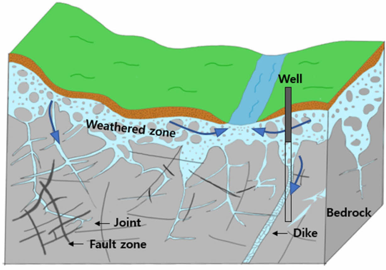
국내 대수층은 상대적으로 심도가 얕은 충적 대수층과 심도가 깊은 암반 대수층으로 구분할 수 있다. 주로 미고결 퇴적물로 구성되어 있는 충적 대수층은 국내 대수층의 28%를 차지하고 있으며, 한강, 낙동강, 영산강, 섬진강과 같은 주요 강들을 따라 분포한다(Lee et al., 2017). 일반적으로 지각 활동에 의해 형성된 단층, 균열, 절리 등이 있는 암반 대수층은(Fig. 2), 일반적으로 얕은 대수층에 의해 덮혀 있다(Lee et al., 2007). 지하수 부존량이 많고 수리전도도도 커 주요한 수자원의 공급원인 충적 대수층들은 농업에 이용된 농약과 비료에 의한 질산염 오염이 많아서(Min et al., 2003), 국내 지하수 중 식수로 사용하는 대부분은 균열 암반 대수층에 의존하고 있다(Min et al., 2002; Chae et al., 2004; Lee et al., 2007).

- 연안 대수층(coastal aquifer)
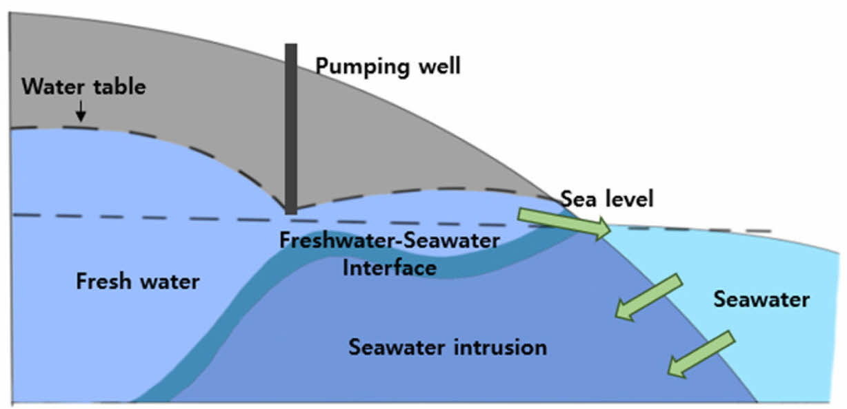
담수 지하수가 주요한 물의 공급원인 연안 지역에서는, 자연 상태에서 내륙에 위치한 담수의 바다로의 이동이 해수가 해안 대수층을 잠식하는 것을 막아 준다. 일반적으로 담수보다 해수의 밀도가 더 높아 담수가, 담수와 해수의 경계 위에 위치하게 되는데(Bear et al., 1999)(Fig. 3), 최근들어 산업 및 농업 분야에서 담수 수요의 증가로 인해 담수 지하수가 무분별하게 개발 사용되고 있어(Hamed et al., 2018
) 해수가 해안 담수 대수층을 잠식하는 경우가 빈번하게 발생하고 있다. 즉, 과도한 지하수 사용으로 대수층 내의 담수-해수 경계에 존재하는 유체역학적 평형의 훼손되어 해수 침투가 유발되며 이로 인해 담수 지하수의 고갈이 발생하고 있다(Alfarrah and Walraevens, 2018).

2.2. 대수층 내 점토 영향
퇴적층 대수층과 그 주변을 이루는 지하매질에 점토가 함유된 경우엔, (불투수성 지층과 같이) 지표수와 지하수의 상호작용을 방해하게 되며(Uhlemann et al., 2017) 특히, 암반대수층에서는 단층비지(fault clay) 또는 단층점토(fault gouge)의 형태로 존재하면서 투수성의 감소를 유발한다(Chae et al., 2001). 점토층의 두께 및 분포를 파악하면 물의 우선 흐름 경로(trace of window)에 대한 파악이 가능해져 지하수위나 대수층 함양(recharge)에 대한 정보를 얻을 수 있다(Uhlemann et al., 2017). 연안 대수층의 경우, 점토가 해수를 함유한 대수층과 담수 대수층을 분리하는 역할을 하기 때문에 점토 분포를 파악하려는 연구도 진행되었다(e.g., Buddemeier et al., 1995). 이와 같이 점토는 여러 대수층에 다양한 영향을 미치기 때문에 대수층 평가에서 점토의 분포를 파악하는 것이 중요하다.

2.3. 전통적인 대수층 특성화 방법
대수층을 특성화 하기 위해 전통적으로 사전조사를 수행하여 대수층 위치를 파악하고 시추공을 이용한 정밀 조사를 수행한다. 사전조사 방법으로 크게 문헌조사, 지표지질조사, 지구물리탐사가 있다. 문헌조사는 인근 지역의 시공 사례나 전문가의 조언을 받아 진행되며, 지형도, 위성사진, 지질도를 참고하기도 한다. 수문현황조사와 지질구조 및 지질분포를 파악하는 지표지질조사를 통해 개발 지점을 선정한 후 물리탐사를 수행하여 대수층 분포 가능성을 확인하기도 한다(MOE, 2020).
사전조사를 통해 대수층의 위치를 파악한 후 대수층 특성화를 위해 시추공을 굴착하여 시료를 채취하거나 대수성시험을 수행한다(MOE, 2020). 국내에서는 대수층 평가를 위해 유역별로 여러 위치에 관측공을 설치하여 지하수위, 함수량(water content), 전기전도도, 수온 등을 모니터링하고 있다(MOE and K-water, 2019; Slater and Binley, 2021). 관측공에서의 자료는 함양량 산정(Kim, 2013), 지하수 시공간적 변동 특성 평가(Kim et al., 2015), 가뭄 지역 지하수 연구(Lee et al., 2018), 수위 변동 예측 및 지구화학적 특성 평가(Chung et al., 2007; Jeong et al., 2017) 등의 대수층 평가 연구에 활용되고 있다. 시추공 조사 외에도, DTS(distributed temperature sensing) 센서를 이용해 온도 분포를 확인하거나 간접적으로 토양의 용적수분함량을 확인하는 TDR(time domain reflectometry)을 이용하기도 한다(Briggs et al., 2012).

대수층을 평가하는 데 주로 적용되어 온 물리탐사 방법에는 매질의 전기비저항(electrical resistivity, ER) 분포를 파악하는 전기비저항 탐사(ER survey/tomography, ERT) (부록 A-1), 자연전위(self-potential, SP) 이상을 측정하는 SP 탐사(부록 A-2), 매질의 유도분극(induced-polarization, IP) 현상을 분석하는 IP 탐사(부록 A-3), 매질의 유전율(electrical permittivity) 분포를 파악하는 지표투과레이더(ground penetrating radar, GPR) 탐사(부록 A-4), 지하의 전기전도도 분포를 측정하는 전자(Electromagnetic, EM) 탐사(부록 A-6), 그리고 진동수 영역 EM 탐사의 한 종류인 자기지전류(Magnetotelluric, MT) 탐사(부록 A-5) 등이 있다. 또한 대수층 지질 분포 해석을 위해 굴절법 탄성파탐사도 활용되었다.

3.1. 대수층 평가를 위한 주요 물리탐사 물성
대수층 특성화에 활용되는 주요 물성은 전기비저항과 유전율이다. 일반적으로 지하수로 포화되어 있는 영역이, 불포화대보다 낮은 전기비저항을 보이므로 전기비저항 분포를 해석하여 대수층 위치를 규명할 수 있다(Saad et al., 2012). 즉, 대수층에서 물이 공극을 채우고 있는 경우 공극률의 증가, 풍화 정도의 증가, 파쇄대 및 균열의 증가로 인해 전기비저항이 낮아지고, 염도, 함수비(water saturation), 점토 함유량이 증가하는 경우에도 전기비저항이 낮아진다(Samouelian et al., 2005; Park et al., 2013). 점토질을 함유한 대수층의 경우, 점토의 표면적은 최대 1000 m²/g로 0.1 m²/g 미만인 모래보다 넓어 표면 전도도가 크고(Waxman and Smits, 1968), 고체와 액체의 경계, 즉 확산 이중층(diffuse double layer) 사이의 상대적으로 높은 전도도로 인해 일반적으로 공극수(공극 유체)에 비해 전기비저항이 낮게 나타난다(Fukue et al., 1999).
유전율은 특히 지하수 포화 토양과 불포화 토양 사이의 유전 특성 차이가 크기 때문에 지하수 탐사에 효과적이다(Schmugge, 1980). 층 경계와 침투 깊이의 반사율을 결정하는 물리학적 매개변수인 물의 유전율은 약 81로 다른 매질에 비해 큰 값으로 나타난다(Chandra, 2019; Yu et al., 2019). 점토 광물의 양이온과 관련된 전기화학적 과정으로 인해 전도성 기반 에너지 손실이 발생하기 때문에(Neal, 2004), 점토가 있는 경우 레이더 신호의 감쇠로 인해 GPR 탐사의 최대 침투 깊이가 감소한다(Abed et al., 2020).

3.2. 대수층 평가를 위해 분석할 수 있는 물리적 현상
IP 반응은 공극 내 유체의 물성과 공극률, 공극의 내부 면적과 같은 공극의 기하학적 특성에 영향을 받기 때문에 수리지질학적 변수와 IP 반응과의 관계성을 설명하고자 하는 연구가 많았다(Leroy et al., 2008; Weller et al., 2015). 점토층은 모래 또는 자갈을 포함하고 있는 다른 층들에 비해, IP 반응을 야기하는 충전성이 높게 나타난다(Cho et al., 2008). 한 층이 같은 양의 점토로 구성되어 있더라도 하나의 두꺼운 사암층보다 여러 층으로 구성된 얇은 사암층에서 IP 반응이 더 크게 나타난다(Draskovits et al., 1990).
SP 탐사법을 이용하여 지하수 유동 해석을 수행할 때는 지하수 유동에 의해 발생하는 흐름 전위 이상대를 수동적으로 측정하는 것을 목표로 하며, 흐름 전위는 지하수의 포화 상태 및 유체 흐름 특성에 따라 달라진다(Song et al., 2021; Ahmed et al., 2020). 점토가 함유된 대수층의 경우, 계면동전 결합 계수(electrokinetic coupling coefficient) 값이 크게 감소하기 때문에 SP 값이 크게 감소하는 것이 일반적이다(Revil et al., 2003). 대수층의 구성물질 중 물로 포화된 층과 포화된 점토층은 다른 층들에 비해 상대적으로 낮은 전기비저항 이상대가 나타나기 때문에 사실상 이들을 전기비저항 탐사만으로 구별하기 어렵다(Van Dam, 1976).

3.3. 물리탐사 기초 수리상수 도출
대수층 특성화를 위한 물리탐사는 주로 기본적인 층서구조, 파쇄대, 점토질 토양 분포 등과 같은 매질 지하매질을 정성적으로 해석하는 경우가 많으나 유체를 포함한 다공성 매질의 전기적 특성을 기반으로 시추공 자료 기반 수리지질 변수와 물리탐사 변수의 상관관계를 이용해 대수층의 수리지질학적 변수를 정량적으로 구하기도 한다(Deiana et al., 2007; Batte et al., 2010; Zhu et al., 2016; Vogelgesang et al., 2020). 또한, 최근에는 물리탐사 자료만을 이용해 수리지질학적 변수를 예측하고자 하는 연구도 활발히 이루어지고 있다(Akhter et al., 2022; Song et al., 2022).

- 수리전도도(K) 및 투수량계수(T) 도출 방법
수리전도도(hydraulic conductivity, K)는 다공성 매질의 공극 내에서 유체의 흐름의 용이도를 나타내는 척도로 지하수의 흐름을 정량화 하는 데 사용되며, 다음과 같이 정의한다.



여기서 k는 유체투과도(혹은 투수율, permeability), d_w는 유체 밀도, μ는 유체 점성도, g는 중력 가속도이다. 대수층의 투수량계수(transmissivity, T)는 수리전도도 K와 두께 b의 관계를 이용하여 다음과 같이 나타낼 수 있다.



Archie 식은 다공성 매질의 공극률, 함수비 및 전기비저항의 관계에 대한 식으로 다음과 같이 나타낼 수 있다(Archie, 1942).



여기서 S_w는 함수비, n은 포화 상수, a는 비틀림 계수, φ는 공극률, m은 고결 상수, R_w는 지층수의 전기비저항, R_f  는 지층의 전기비저항이다. 대수층의 투수량계수를 수리전도도 K와 전기비저항 ρ의 관계를 이용하여 종방향 수리 흐름 및 횡방향 수리 흐름과 전류에 대해 대수층 투수량 계수를 각각 다음과 같이 나타낼 수 있다.



여기서 ρ는 전체 전기비저항(bulk resistivity), S는 두께 b로 나타낸 대수층의 종방향의 전도도(longitudinal conductance)이며, b/ρ이다. 여기서 R은 대수층의 횡방향 저항도(transverse resistance)이며, bρ이다. 이때 만약 대수층이 균일한 전기비저항의 물로 포화되어 있다면, Kρ,K / ρ가 일정하게 유지될 것이다. 따라서 위의 식은



여기서 a, β는 비례 상수이다. 이와 같은 방법으로 수리상수와 전기비저항 사이의 상관관계를 선형 회귀를 통해 구할 수 있다.
위 식들을 적용하기 위해서는 K, T 같은 수리상수값과 ρ 같은 전기적 측정 값 사이의 비례상수 값을 유추하는 과정이 필요하다. 하지만 σ'은 공극 내 유체의 전기전도도와 다공성 매질 알갱이의 경계면 전기전도도에 모두 영향을 받기 때문에 이를 분리하여 분석하기 쉽지 않아 K 값을 예측하는 데 명확한 한계가 있다.
실수 전기전도도만을 이용할 경우 얻을 수 있는 정보의 한계점은 매질의 전기전도도와 충전 효과 특성을 같이 측정하는 IP 탐사 혹은 복소 전기비저항(complex resistivity; CR) 탐사법을 통해 해결할 수 있다. 허수 전기전도도(σ''; [mS/m])가 상호 연결된 공극 표면적에 대한 특성에 유일하게 관여된 변수라는 사실 때문이다. Börner et al. (1996)은 전기전도도 허수성분과 k의 선형관계를 제시하였으며 이를 기반으로 IP 변수로부터 수리전도도를 예측하고자 하는 많은 연구가 수행되고 있다(Börner et al., 1996; Slater and Lesmes, 2002; Slater et al., 2006) (부록 B 참조).
한편, 자연 전위 지배방정식에서의 단위 공극 부피당 과전하 Q͞͞_v와 유체투과도 k의 관계를 이용하는 방법으로도 유체투과도를 유추해볼 수 있다. 먼저 자연 전위 지배방정식은



이며(Revil and Leroy, 2004; Revil and Linde, 2006), 여기서 u는 Darcy velocity [m/s], j는 전류밀도, E는 전기장,s는다공성 매질 전기전도도[S/m]이다. 정상 상태에서 전류의 발산이 0인 것으로부터 흐름 전위 송신원 S͞͞는



으로 표현할 수 있으며(Song et al., 2021), 정량적 해석으로부터 전류원을 역해석할 수 있다(Bolève et al., 2007). 위 식에서 Q͞͞_v는 아래와 같이 유체투과도와 관계식으로 표현될 수 있는데,



이때, C는 계면동전 결합 계수, n_f 는 공극수의 동적 전단 점성(dynamic shear viscosity) [Pa·s]이다. 흐름 전위 역산 결과에서 Q͞͞_v 값을 평가하고 (8)식으로부터 유체투과도와 누수 속도와 같은 수리 상수를 평가하는 연구도 수행 중에 있다(Bolève et al., 2007; Ahmed et al., 2019). 또한 다양한 매질에서의 Q͞͞_v와 k의 관계를 실험식으로 나타내기도 하였다(Bolève et al., 2012).



여기서 a와 b는 각각 9.9956, 0.9022이며, 이 값은 Bolève et al.(2012)이 보다 넓은 범위의 유체투과도 분포에서 성립 가능할 수 있도록 보완한 결과이다(Song et al., 2021).

4.1. 전기비저항 탐사
ERT 탐사는 지하수 자원 평가에 유용하고 파쇄 및 단층 구역, 높은 다공성 및 투과성 구역과 같은 지하수의 잠재적 구역을 식별할 수 있다(Owen et al., 2005; Sharma and baranwal, 2005; Kumar et al., 2020). 한편 복잡한 지질학 및 수리지질학 분야에 전기비저항 탐사를 적용하기 위해 저항 특성에 대한 2D 및 3D 고해상도 영상화 기법을 발전시켰다(e.g., GrifBths and Barker, 1993; Daily et al., 2004; Gokturkler et al., 2008; Thiagarajan et al., 2018; Swileam et al., 2019). 수직 전기비저항 탐사(vertical ER survey; VES)는 수평 전기비저항 분포의 해상도가 상대적으로 좋지 않아 복잡한 지질 모델에서 적용하기에 적절하지 않지만(Griffiths and Barke, 1993) 대수층 목표 심도에 따라 목표 심도가 깊을 경우, 수직 전기비저항 탐사를 수행하여 한 지점에서의 정보를 영역 전체에 걸쳐 공간 보간하여 대수층 특성화에 활용한다(Ahmed et al., 1988; Soupios et al., 2007; Sattar et al., 2016; Hasan et al., 2018). VES 탐사에 의해 넓은 지역에서 확인된 지하수 구역은 시추공을 뚫어 한 지점에서 확인하여 신뢰성을 높일 수 있다(Rai et al., 2013).

4.2. 자연전위 탐사
SP 탐사는 다공성 매체의 공극수 흐름에 의해 야기되는 자연 전기 전위 이상을 측정하는 수동적 지구물리탐사 방법으로 측정하기 쉽고 비용도 효율적이라는 장점이 있다. SP 탐사로 측정된 전위는 원인이 되는 전류원을 결정하고 지하수 흐름, 수리역학적 및 지구화학적 정보를 얻는 데 사용될 수 있다(Revil and Jardani, 2013). SP 조사는 다른 물리탐사 방법과 결합하여 지하수 흐름과 오염물질 확산의 국지화 및 정량화와 지하수면, 유체투과도와 같은 대수층과 관련된 수리적 특성을 추정하는 데 특히 유용하다. 유역에서는 음(-)의 SP 이상대, 유출 영역에서는 양(+)의 SP 이상대를 보이며, 특히 유량이 클수록 음의 전위의 진폭이 증가하는 특성을 가진다(Ahmed et al., 2020; Panthulu et al., 2001; Naudet et al., 2003).

4.3. 유도분극 탐사
IP 탐사법은 지하에 일정시간 동안 전류를 보낸 후 전류를 끊고 전위차를 측정하여 충전성을 측정하는 시간영역 유도 분극 탐사와 두 개 이상의 진동수에 대한 진폭 및 위상을 측정하는 광대역 유도분극 탐사로 나눌 수 있다(Reynolds, 2011). IP 탐사는 매질의 입자와 공극 유체 사이의 표면에서 발생하는 분극에 의한 충전성이나 여러 변수를 측정함으로써 점토를 구분하거나 전해질을 포함한 지하수 탐사, 염수 침입에 영향을 받은 토양 대수층 평가에 적용할 수 있다(Slater and Lesmes, 2002; Cardarelli and Filippo, 2009; Atekwana et al., 2010).
IP 탐사는 전기비저항 탐사와 같은 전극 배열을 사용할 수 있기 때문에(Revil et al., 2012; Madun et al., 2018) 전기비저항 탐사 결과 저비저항 이상대가 나타나는 경우 IP 탐사를 수행한 결과로 추가적인 물성 정보를 얻어 이상대의 원인 해석에 신뢰성을 높일 수 있다. 특히 진동수영역에서 IP 반응을 측정하는 복소전기비저항 혹은 광대역 유도분극 탐사(spectral IP; SIP)법은 유체투과도에 큰 영향을 끼치는 수리적 변수와 관계성이 밝혀지면서 큰 주목을 받게 되었다. 공극 내 유체의 특성에 대해서만 주로 분석할 수 있는 전기비저항과 달리 IP 반응은 공극률, 내부 면적과 같은 공극의 기하학적 특성(pore space geo- metry)과 유체의 염분 등으로 결정되는 공극 내 유체의 물성에 모두 영향을 받기 때문에 실질적인 유체투과도를 결정하는 수리지질학적 변수와의 관계성을 더 잘 설명할 수 있다(Weller et al., 2015).

4.4. 지표투과레이더 탐사
GPR 탐사는 전자기파 중 레이더파를 송신원으로 매질의 물리적 특성에 따라 반사되는 파를 수신하는 방법으로 탐사 심도가 낮으나 상대적으로 높은 해상도의 이미지를 얻을 수 있는 탐사로(Davis and Annan, 1989) 수리 지질학 분야에도 광범위하게 활용되고 있다(Hubbard et al., 1997; Gloaguen et al., 2001; Lesmes et al., 2002). GPR 탐사는 주파수 영역으로 바꾸어 탐사하고 분석할 수 있기 때문에 이러한 특성을 살려서 더욱 신뢰성 높은 탐사를 수행할 수도 있다.

4.5. 전자 탐사
EM 탐사는 1차장에 의해 지하에 유도되는 유도전류에 의한 2차장 또는 합성장을 측정하여 지하의 전기전도도 분포를 파악하는 방법으로 크게 주파수 영역 EM 탐사(frequency-domain EM, FEM)와 시간 영역 EM 탐사(time-domain EM, TEM)로 나눌 수 있다. 전기비저항 탐사에 비해 EM 탐사는 지면과 직접 접촉할 필요가 없으며, 고저항성 매질에서는 높은 투과율, 고전도성 매질에서는 높은 해상도를 제공한다는 장점을 가진다(Macnae and Nabighian, 1987). 토양의 전기 전도도는 수분 함량과 염분 함량뿐만 아니라 토양 구조, 질감, 광물학과 관계도 가지고 있기 때문에(Nadler and Frenkel, 1980; Shainberg et al., 1980), EM 탐사는 전기전도도 분포를 파악하여 지하 매질에서 균열대를 찾거나 지하수를 찾는 데 활용된다. 또한 TEM과 ERT 자료의 복합 역산(joint Inversion)은 TEM 또는 ERT만으로 얻은 분해능과 비교하여 지층 구조의 분해능을 크게 개선할 수 있다(Raiche et al., 1985).

4.6. 자기지전류 탐사
MT 탐사는 FEM에 속하는 방법으로, 지구의 자연 전자기장을 사용하여 수십 m에서 수십 km 깊이까지의 전기 전도도 분포를 조사하는 수동적 지구물리학적 방법으로, 전자기파의 관계에 의해 수직적 및 수평적 변화에 민감하여 MT 탐사는 복잡한 지질학적 구조를 연구하기에 적합하다(Vozoff 1972). 특히 가청주파수 MT(audio frequency MT; AMT) 탐사는 중층 및 얕은 지층의 구조를 탐지하기 위한 일반적인 수단으로 수자원 조사에 사용되어 왔다(Yu et al., 2014).

지하 암반 대수층에 부존 되어 있는 지하수를 탐지하거나 정확한 위치를 규명하기 위해 수행된 물리탐사 사례들을 소개하고 탐사 결과들에 대해 분석하고자 한다.

5.1. 대수층을 가지는 대표적인 지질구조에서의 적용 사례
균열 암반 대수층은 국내 뿐 아니라 해외에서도 상당히 중요한 의미를 가지게 되며 이에 따라 균열 암반 대수층을 규명하기 위해 각종 지질조사, 물리탐사 및 수리지질조사를 수행하고 있다(Watlet et al., 2018). 또한 국내 대다수의 대수층이 형성되어 있는 충적층은 수자원 확보를 위한 인공함양 대상지로도 활용되며, 지하수 이용을 위해 대수층 평가가 필수적이다(Won et al., 2013). 일반적으로 전기비저항은 공극률, 광물의 함량, 지하수 흐름 등의 많은 요인에 의해 지배되고, 지층의 풍화상태 및 파쇄대의 존재에 따라 달라지기도 한다. 파쇄대는 주변보다 공극률이 크기 때문에 물로 포화된 경우 파쇄대 부분의 전기비저항이 상대적으로 낮아지고, 특히 점토를 많이 함유한 파쇄대의 전기비저항은 명확하게 낮은 이상대를 보인다(Lee et al., 2001; Watlet et al., 2018).
충전성과 같은 IP반응은 막분극에 의해 침전물이나 암석에 점토 광물이 존재할 때 발생하기 때문에 점토가 포함되어 있는 매질에서는 저비저항 이상대가 나타나는 경우 지하수 분포 해석에 신뢰성이 떨어질 수 있으므로 IP 탐사 자료와 함께 해석하여 신뢰성을 높일 수 있다(Madun et al., 2018). 한편 GPR 탐사 자료에서는, 물로 채워진 균열 암석은 낮은 진폭의 반사 영역으로 단면에 나타나고, 파형 위상 극성와 유전상수의 대비를 분석하여 물의 존재를 결정할 수 있다(Travassos et al., 2004; Nakashima et al., 2001; Liu et al., 2014).

- 지하수 부존이 예상되는 파쇄대 탐지 사례
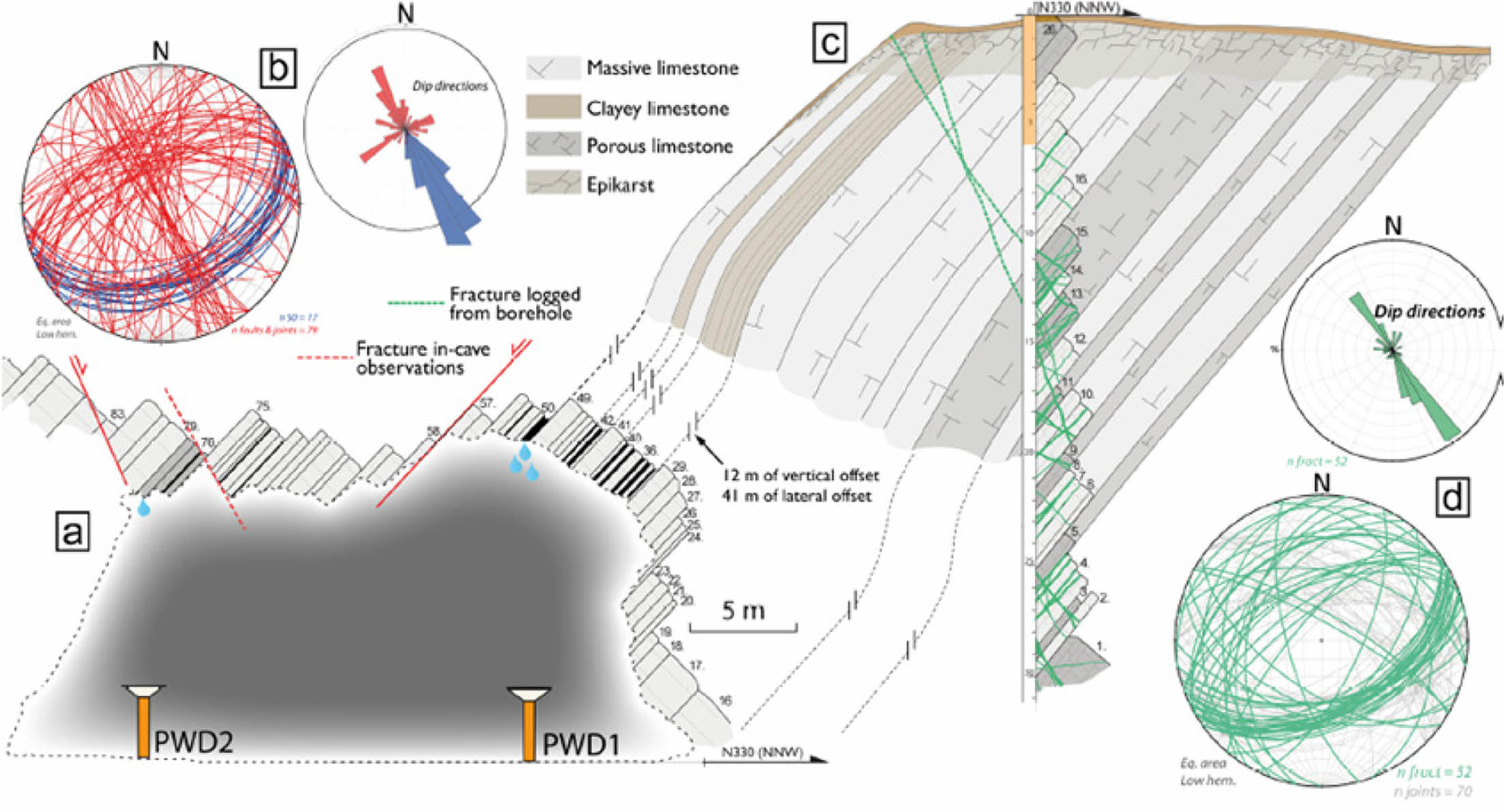
대표적인 사례로 벨기에 카르스트 지역(karst area)의 지하수 부존 위치를 파악하기 위해 계절 변화에 대한 영향을 확인하기 위해 전기비저항 시간경과 모니터링을 수행한 사례가 있다(Watlet et al., 2018). 탐사는 4-채널 Iris Syscal Pro를 사용하였으며, 분해능을 고려하여 쌍극자 배열과 기울기 배열을 사용하였다. 시간경과 모니터링 결과 증발산량의 증가로 봄과 여름에 높은 전기비저항이 나타났으며, 불포화대의 지하수 함양으로 겨울에는 낮은 전기비저항이 나타났다(Fig. 4). 전기비저항 탐사와 더불어 국지적 규모의 상세한 구조를 알기 위해 시추공 탐사를 실시하고, 복합 해석한 결과 낮은 전기비저항이 나타나는 곳과 파쇄대의 방향이 일치함을 확인하였다(Fig. 5).
화강암 지역에 선구조(lineament)가 존재하는 곳에 측선을 설정하여 GPR 탐사와 2차원 전기비저항 탐사를 복합적으로 탐사하였으며, 담수와 점토를 구분하기 위해 추가로 감마선 분광법, 라돈가스 방사 측정기법을 수행한 사례가 있다(Porsani et al., 2005). GPR 탐사는 100 MHz의 안테나를 사용하여 wide angle reflection and refraction (WARR)기법으로 20 m 깊이까지 수행하였으며, 전기비저항 탐사는 쌍극자 배열을 사용하여 30 m 깊이까지 수행하였다. 물과 화강암 사이의 강한 유전 상수의 대조로 높은 진폭이 나타나기 때문에 물로 채워진 경사 균열에서 쌍곡선 반사가 나타났다. 전도성이 높은 곳은 신호 감쇠가 심해지므로 물이나 점토로 채워진 수직 파쇄대에 해당하는 곳에서는 명확한 신호를 보였다. 신호 감쇠 영역은 전기비저항 탐사 결과 낮은 전기비저항을 보이는 곳과 일치하였다.
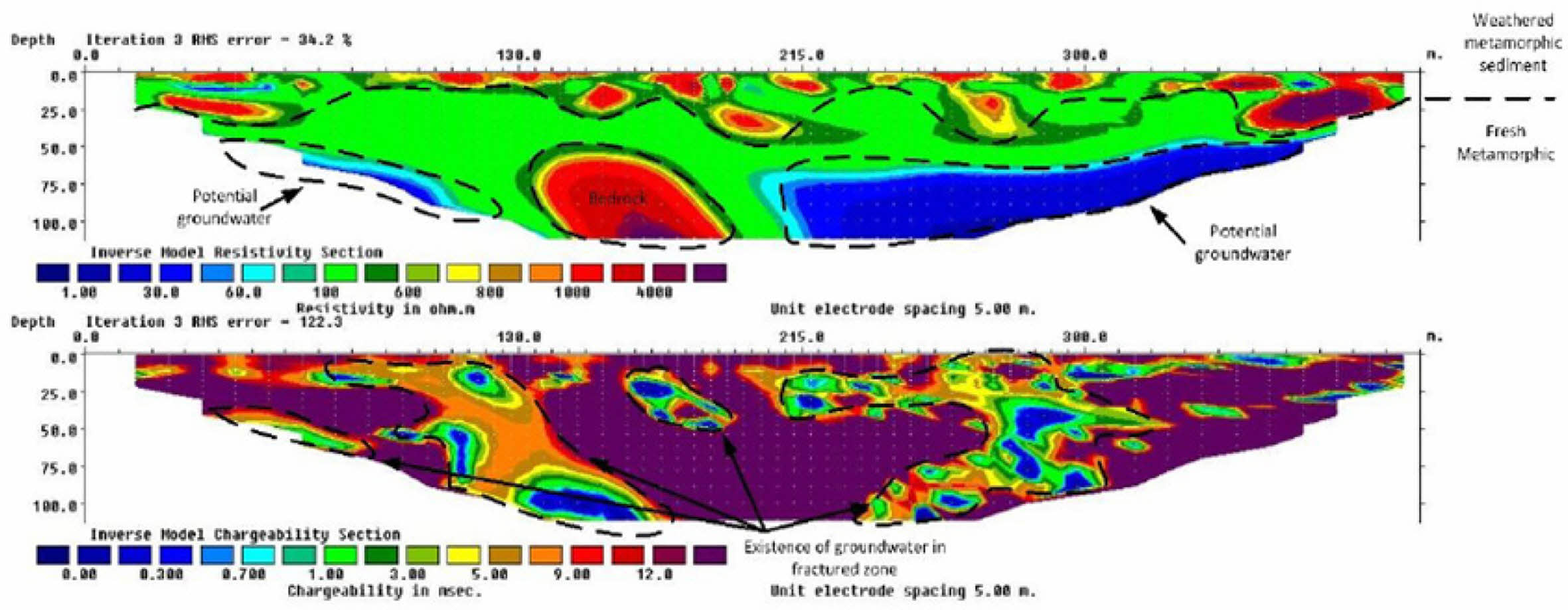
지하수와 점토를 구별하기 위해서 전기비저항 탐사 수행 후 시간영역 IP 탐사를 추가적으로 수행하기도 한다(Aizebeokhai et al., 2014; Madun et al., 2018). 두 탐사 모두 직류 송신원을 사용하기 때문에 동시에 수행하고 해석하기도 한다. 점토가 포함된 층의 경우 IP 반응이 증가하기 때문에 대수층과 점토층을 효과적으로 구분할 수 있다(Fig. 6).
인도의 화강암질 지역인 하이데라바드에서 지하수가 존재할 확률이 큰 파쇄대를 찾고 지하수 잠재 구역을 규명하기 위해 GPR 탐사, 지표 전기비저항 탐사, VES 탐사를 수행한 후 시추공 탐사를 수행할 위치를 선정하였다(Sonkamble et al., 2013).

- 충적층 지역에서 지하수위 추정 사례
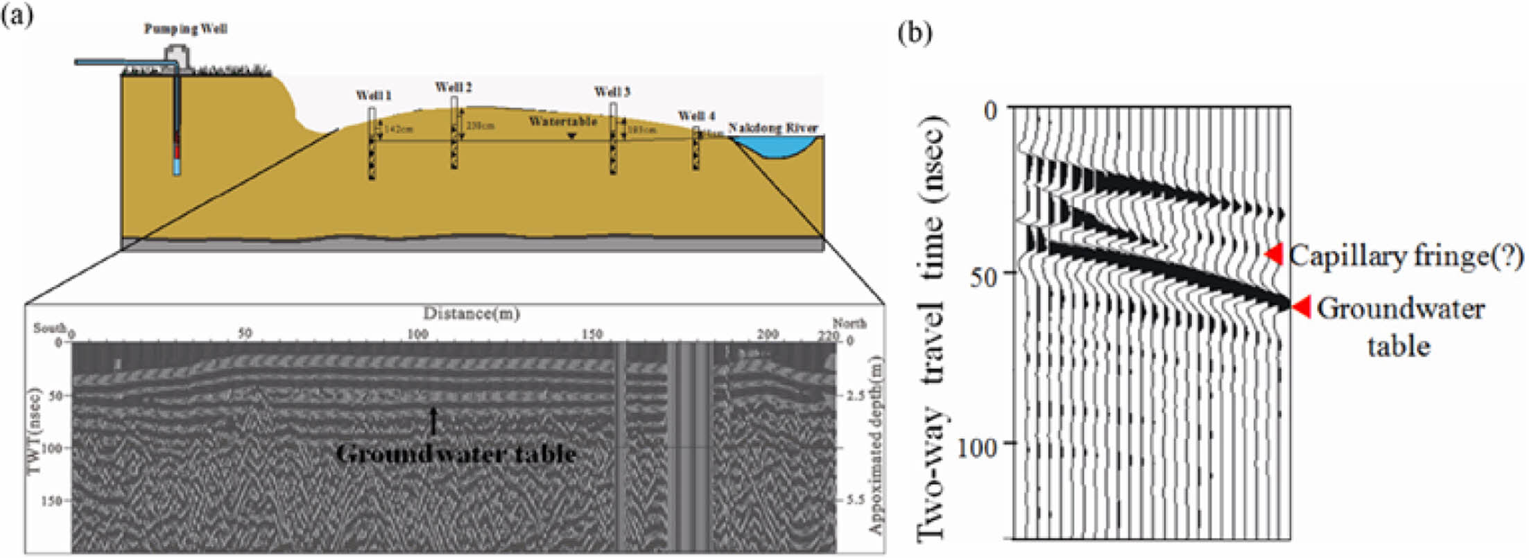
낙동강변 충적층에서 지하수위를 추정하기 위해 GPR 수직반사법(Vertical reflection profile, VRP)과 중앙공심점(common mid-point, CMP) 탐사를 수행하였다(Kim et al., 2013). VRP 탐사는 탐사심도를 10 m로 설정하여 지하수위를 파악하기 위해 100 MHz 안테나를 사용하였다. CMP 탐사 또한 VRP와 동일한 안테나를 사용하였으며, 송수신 안테나 간격을 0.2 m씩 양방향으로 이동하는 방법으로 수행하였다. VRP 탐사 결과, 잔류포화대와 모관대를 통과하는 레이더의 속도가 감쇠하여 왕복 주시에 의해 계산된 지하수위의 심도가 흐릿한 반사면을 보이며, 뚜렷하게 구분하기 어렵게 나타났다(Fig. 7a). CMP 방법으로 수행한 탐사 결과, VRP 결과보다 뚜렷하게 지하수면의 경계를 추정할 수 있었다(Fig. 7b). 종합적으로 현장에서 해석한 지하수위는 관측공을 통해 얻은 지하수위보다 다소 낮았는데 이는 점토질 층들로 인해 부분적으로 피압으로 관측공 설치시 형성된 피압의 결과로 해석하였다.
충적층 내의 점토의 분포 및 대수층을 함유하는 모래자갈층의 저기저항 분포를 해석하기 위해 전기비저항 탐사와 수직탐사를 이용하여 대수층을 탐사할 수 있다(Won et al., 2013). 전기비저항 탐사는 Supersting R8/IP 장비를 이용하였으며, 심도가 깊은 곳에서는 분해능의 저하를 고려하여 가탐심도를 정한 후 자료처리하였다. 수직탐사의 장점인 수직 분해능과 2차원 전기비저항 탐사의 수평 분해능을 비교 분석하여 충적층 내부 구조를 파악하고 점토층 위치와 대수층 두께 및 지하수위를 추정하였다.
충적층이 해안가에 위치한 오만(Oman)의 경우, 염수 침투 영역을 조사하고자 시간영역 전자탐사를 수행하였다(El-Kaliouby and Abdalla, 2015). 탐사 전 배경조사를 통해 조사지역은 지표로부터 300 m까지 충적층으로 구성되어 있으며, 일부 구간은 최대 600 m 깊이 까지 충적층인 것으로 조사되었고, 매질은 큰 사이즈의 자갈이 주를 이루는 것으로 나타났다. 1D 역산 결과, 남북방향 측선에서 바다와 약 2 km 떨어진 구역에서 매우 낮은 전기비저항이 나타났으며, 이를 염수에 의해 나타난 결과로 해석하였다. 동서방향 측선에서도 염수의 침투에 의한 낮은 전기비저항을 확인할 수 있었다.

5.2. 해안 대수층에서 담수 및 염수를 구분하여 지하수를 특정하는 사례
많은 해안 대수층은 해수 침입에 취약하며, 많은 지역에서 수많은 발생 사례가 보고되고 있으며, 이러한 해수 침투에 의한 지하수 염수화로 많은 지역에서 지하수 개발에 어려움을 겪고 있다(Barlow and Reichard, 2010; Bocanegra et al., 2010; Custodio, 2010; Morgan and Werner, 2015; Shi and Jiao, 2014; Steyl and Dennis, 2010). 해수 침입을 특성화하고, 담수와 구별하기 위한 기존 방식은 시추공 수리화학(hydrochemistry) 및 지하수위 모니터링, 물리탐사 방법으로 총 세가지로 분류된다(Werner et al., 2013). 시추공 수리화학 및 모니터링 방법은 불균질(heterogeneous) 대수층에서의 해수 침투 특성화를 해석하는데 한계가 있다. 따라서 시추공 탐사를 대체할 수 있는 방안으로 물리탐사 방법이 필요하며, 주로 전기전자 탐사법을 이용한 해수 침투 특성화가 일반화되고 있다(Comte and Banton, 2007; Fitterman, 2014).
염수에서의 전기비저항이 담수에서의 전기비저항 보다 값이 낮아진다는 점을 이용하여 전기비저항 탐사를 수행한다. 대표적인 사례로 이집트 홍해 연안 지역에서 염수와 담수를 구분하여 식수를 얻기 위한 양수정 위치를 선정하기 위해 VES 탐사를 활용하였다(Mohamaden et al., 2017). VES 탐사 결과를 InterpexIX1D-v.2 소프트웨어를 사용하여 자료 처리하여 등고선지도를 그려 해석한 결과 해안가와 맞닿아 있는 동쪽은 염수로 인해 낮은 전기비저항이 나타났으며, 서쪽은 담수의 존재로 상대적으로 높은 전기비저항이 나타난 것을 확인할 수 있다. 국내에서는 염수침투 피해를 개선하고자 충적층 및 균열 암반 지역에서 담수를 주입하고 전기비저항 탐사, 자연전위 모니터링, 물리검층과 같은 물리탐사 방법을 수행하여 주입시험의 효과와 지하수 거동을 모니터링한 사례가 있다(Park et al., 2007; Shin and Byun, 2010). 담수를 주입한 후 시간에 따라 전기비저항이 증가하는 것을 확인할 수 있었다(Fig. 7).
각 VES를 수행한 지점에서의 1D 전기비저항 결과를 2D로 확장하여 그려볼 수 있지만 1D에서 2D로 확장하여 그린 그림은 공간적 변동성을 감안하면 완전한 정보를 제공할 수 없으므로 GPR 탐사를 수행하여 수평적 범위를 추정할 수 있다(Tronicke et al., 1999). 따라서 수직 전기비저항 탐사와 GPR 탐사를 복합 해석하여 더 정확한 지하수 정보를 얻을 수 있다.
AMT 탐사 역시 전기비저항 분포를 파악하여 대수층에서의 해수 침입 정도를 해석할 수 있다(Ritz et al., 1997). AMT sounding 탐사를 수행하여 1-D 전기비저항 분포를 확인한 결과, 3 ~ 10 ohm-m 범위의 전기비저항 층을 전도성이 강한 염수로 포화된 현무암층으로 해석하였다. 담수로 포화된 층은 100 ~ 1000 ohm-m로 해석해 개략적인 담수의 깊이를 추정해볼 수 있었지만 정확한 위치를 판별하기 어렵다고 판단하였다. 비록 기저 대수층을 전기적으로 뚜렷하게 판별할 수 없었지만 중간 저항층의 하부를 대수층의 주체를 구성하는 담수 포화 물질로 구성되어 있을 것이라 해석할 수 있다.
해안가에서 담수, 염수 interface의 구조를 조사하기 위해 전기비저항 탐사를 수행하고 추가적으로 시간 영역 IP 탐사를 수행하였다(Slater and Sandberg, 2000). 전기비저항 탐사 결과, 염수와 담수의 interface에서 높은 전기비저항과 낮은 전기비저항의 대조가 나타났다. IP 탐사 결과 표석점토가 존재하는 곳에서 충전성이 높게 나타났지만 염수에서는 상대적으로 IP 반응이 나타나지 않기 때문에 충전성이 없거나 무시해도 될 정도로 나타났다.

5.3. 수리상수 도출 물리탐사 사례
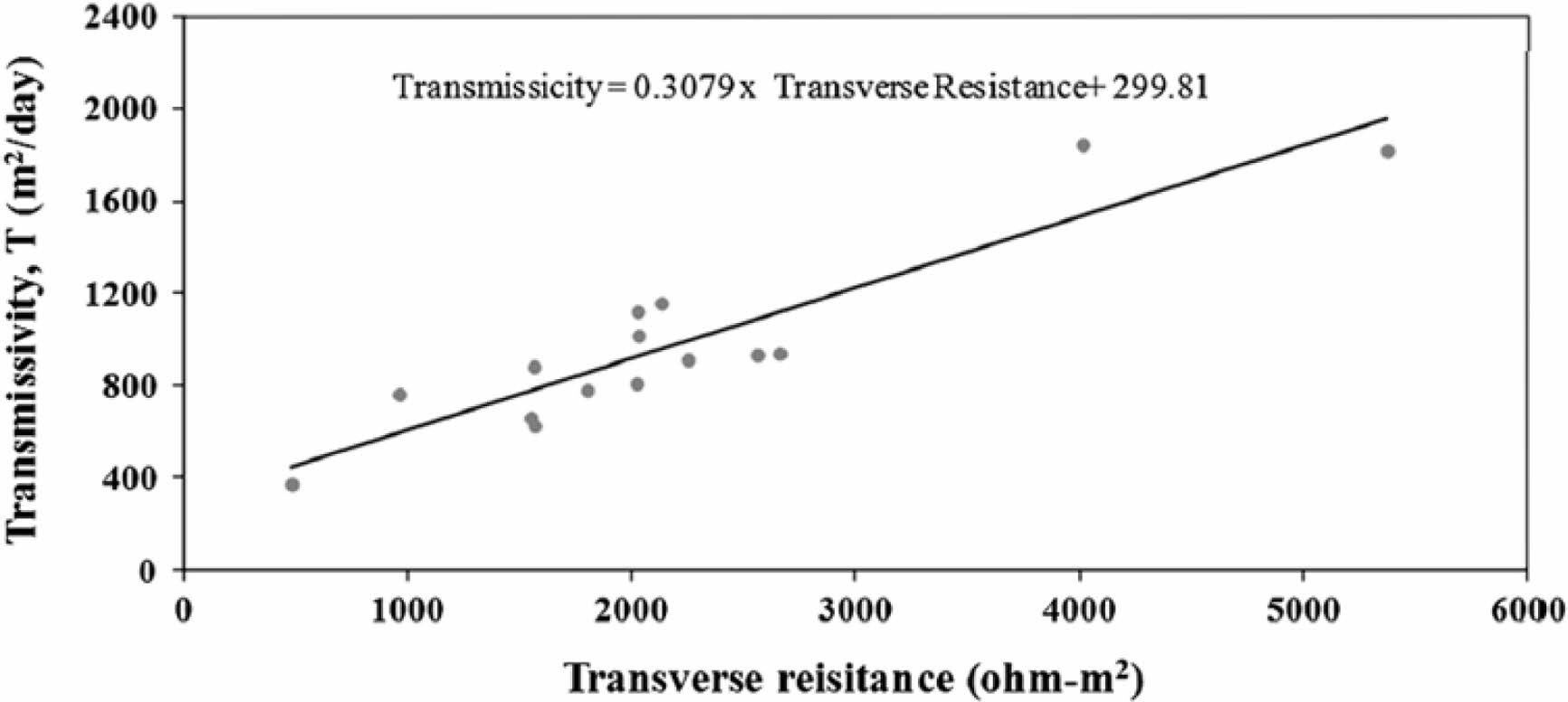
일반적으로 수리전도도와 투수량계수와 같은 수리상수는 현장에서 코어를 획득하여 실내실험을 통해 구하거나 시추공 탐사를 통해 획득되지만 VES 탐사로부터 획득한 전기비저항 데이터를 통해 이를 예측할 수 있다(Sinha et al., 2009; Sattar et al., 2014; Etete et al, 2017; Guevara et al., 2017; Vogelgesang et al., 2020). 따라서 시추공에서 지하수 샘플을 획득해 전기비저항을 측정하고, 현장의 여러 지점에서 양수시험을 통해 투수량계수 및 수리전도도를 측정한다. 또한 VES 탐사를 수행하여 대수층의 두께와 전기비저항 값을 측정하고, 이후 양수시험을 통해 얻은 수리상수와 대수층의 전기비저항의 관계를 회귀하여 관계식을 얻어 수리상수를 추정한다(Fig. 8). 결과적으로 VES 탐사 결과로 수리상수를 도출하여 대수층의 유압 특성을 고려하여 정량적으로 지하수 양수 가능성을 판단할 수 있다.
투수계수는 전기비저항과 물리적인 지배 조건이 비슷하여 공극률 및 파쇄대의 유무, 풍화정도, 점토의 유무, 절리의 발달 정도에 주로 영향을 받는다(Lee et al., 2003). 이를 이용한 대표적인 사례로 국내에서 전기비저항-투수계수의 관계식을 도출하기 위해 양산시 웅상읍 일대에서 전기비저항검층과 수압시험을 수행하였다. 특정 심도에서 수압시험 결과로 나타난 투수계수와 해당 심도의 전기비저항검층 평균값을 도시하여 서로 반비례 관계에 있음을 확인하는 관계식을 구하였다. 연구지역이 해발고도가 높은 산을 관통하고 있으며, 지형이 험하기 때문에 전기비저항탐사가 아닌 가탐심도가 깊은 AMT 탐사를 수행하였다. AMT 탐사는 IMAGEM system을 사용하였으며, 쌍극자 간격을 10 m, 측점간격을 50 m로 설정하여 전기장과 자기장을 측정하였다. AMT 탐사로 얻은 전기비저항 단면도에 전기비저항-투수계수 관계식을 적용하여 투수계수 분포 단면으로 변환하여 이를 지하수 유동모델링에 사용하였으며, 이를 활용하여 대수층 해석을 용이하게 할 수 있다.
인도의 경우, 충적 대수층에서 전기적 특성으로 수리상수를 도출하기 위해 두 곳의 범람원에서 VES 탐사와 양수 시험을 수행하고, 등방성 대수층과 이방성 대수층에서의 모델을 구축하였다(Sinha et al., 2009). 탐사를 수행하기 위해 슐럼버져 배열로 46개의 전극을 사용하여 최대 전극 간격 800 m로 설정하여 VES 탐사를 수행하여 얻은 전기비저항 값과 각 층의 두께와 같은 전기적 특성과 양수 시험으로 얻은 수리상수와 상관관계를 분석하였다. VES 탐사는 양수정과 가까운 지점을 선정하여 수행하였으며, 점토와 대수층 구분을 위해 11지점에서 IP sounding 탐사를 보조적으로 수행하여 해석하였다. 등방성 대수층에서 수리상수 도출을 위해 두 지역에서 횡방향 전기비저항을 계산하여 양수시험으로 획득한 투수량계수와 선형회귀하여 관계식을 얻었다. 이방성 대수층에서 수리상수를 예측하기 위해서 수리전도도, 종방향 전기비저항, 횡방향 전기비저항, 수리 이방성을 포함한 모델을 만들어 계산하였다. 상관관계 분석과 모델을 세워 수리상수를 예측해볼 수 있었으며, 실험값과 비교하여 예측한 값을 검증하였다.
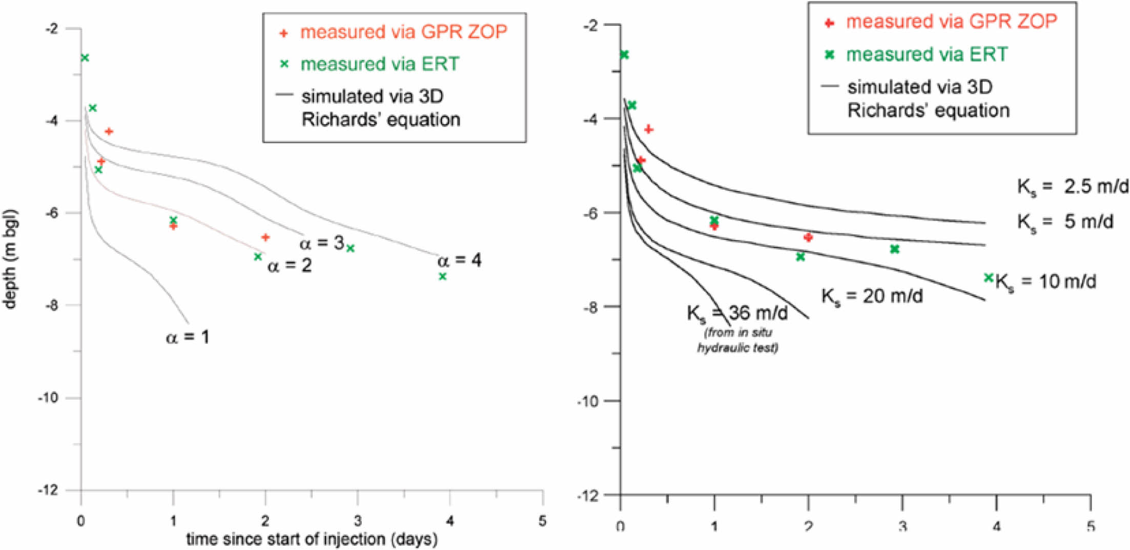
자유면대수층에서 수리전도도를 도출하기 위해 물을 주입 후 시간 경과 시추공 GPR 탐사, 전기비저항 탐사를 수행하고, 그 결과와 수리전도도 별 3D 시뮬레이션을 비교하여 수리전도도를 예측하였다(Deiana et al., 2007). 실험을 위해 3.5 m³ 담수를 주입하고, 3개의 시추공에서 96시간 동안 시간경과 전기비저항 탐사와 zero-offset-profile (ZOP) 기법으로 시추공 GPR 탐사를 수행하여 시간 별 물의 수직 흐름을 해석하였다. 등방성 수리전도도를 사용한 FEMWATER(Lin et al., 1997) 3D 시뮬레이션으로 파악한 질량 중심 수직 운동을 물리탐사 결과와 비교하여 수리전도도를 예측하였다. 물리탐사와 시뮬레이션 비교 결과, 5~10 m/day로 예측할 수 있었다(Fig. 9).
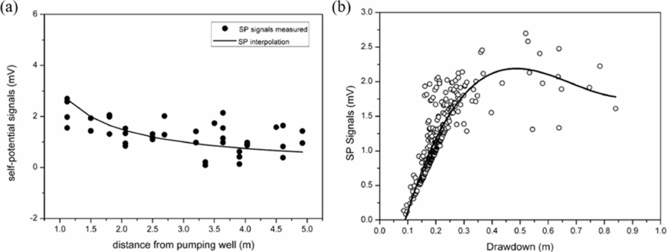
실내 SP 실험을 수행하여 얻은 결과로 균질 다공성 매체의 지하수면 위치와 수리전도도를 추정할 수 있다(Straface et al., 2010). 0.063~0.125 mm 입자 분포의 균질한 석영질 모래(95% 이산화규소)가 채워진 실험용 탱크에 17개의 시추공을 설치하고, 양수정과 배수 파이프를 가장자리에 위치시켜 63개의 Pb-PbCl₂ 비분극 전극을 사용해 SP 탐사를 수행하였다. 양수 전, 후의 지하수위 간 수직적 차이(drawdown) 즉, 수위저하와 SP신호 측정 결과 수위저하가 증가할수록 SP신호도 증가하였으며, 양수 흐름 속도가 낮은 0.4 m의 수위저하까지 선형적인 관계가 나타났다(Fig. 11). SP 전위를 양수정과의 거리, 계면 동전 결합 계수, 수리전도도, 수두, 유량으로 나타낸 방정식(Rizzo et al., 2004)과 양수정과의 거리와 SP 전위를 회귀하여 수리전도도를 추정하였다(Fig. 10).

5.3. 지하수 모니터링 사례
기존의 수리지질적 탐사를 이용한 모니터링 방법은 압력, 온도 변화와 추적자 시험, 시추공 조사 등을 이용하며 이러한 방법들은 보다 세밀한 지층 구조나 지하수의 지역적 변동 특성에 대한 정보를 획득하기는 어려움이 있다(Bai et al., 2021). 지하수 유동 모니터링은 지하수 관리와 오염 방지를 위해서 매우 중요하며, 물리탐사 결과를 2D 또는 3D 영상화 하거나 시간경과(time-lapse) 모니터링하기도 한다(Hayley et al., 2009; Monego et al., 2010; Zhang et al., 2021).
대표적인 사례로 hyporheic(지표수와 지하수 사이의 흐름이 교환되는 곳), riparian(강둑)에서의 수리 지질학적 특성을 파악하기 위해 ERT 탐사, DTS(Distributed tem- perature sensing), GPR 탐사를 수행한 결과이다(Busato et al., 2019). 단기간 시간경과 전기비저항 측정 결과 하상 아래의 전기비저항 분포의 변화가 나타났다. 또한 지표 근처의 전기비저항 증가는 그 시간대의 강수의 부족과 강한 증발로 판단되었으며 저비저항의 분포와 측정한 강의 수위와 비교하여 hyporheic의 하부 구조를 특성화할 수 있을 뿐 아니라 시간당 발생하는 변화를 모니터링 할 수 있었다. 더불어 빙하가 녹아 흘러 들어오는 이 지역의 특성상 DTS를 수행하여 온도 분포를 파악하여 강의 수위와 비교하였으며, 최종적으로 ERT, TDS, 강의 수위 측정을 비교함으로써 다른 방법으로는 파악하기 힘든 hyporheic, riparian 구조도 파악할 수 있었다.
양수시험을 진행하는 동안의 지하수위 변화를 모니터링 하기 위해 시간경과 전기비저항 탐사와 SP 탐사가 이루어졌다(Bai et al., 2021). 전기비저항 결과는 RES2DINV를 사용하여 ERT 역산을 수행하였으며, 시간경과 자료를 얻기 위해 1시간 간격으로 20시간 이상 ERT 모니터링하여 자료를 획득하였다. 그 결과 양수 시험을 진행하면서 저비저항 영역이 심부층으로 이동하는 것을 통해 지하수위가 낮아지고 있음을 알 수 있었다. SP는 양수시험 시 지하수의 흐름에 의해 생성되며, 양수 시험 동안 양수정에서 지하수위가 감소했기 때문에 부분적으로 음의 이상대가 나타난 것을 관찰할 수 있었다. 양수 시험이 종료된 후 전위(potential) 이상대 감소에 따른 여러 양의 이상대가 나타나는데, 이는 함양구간에서 지하수가 흐르며 다시 지하수위가 회복되는 것을 알 수 있다. 이와 비슷하게 국내에서는 양수시험 전후 변화를 관찰하고, 대수층 특성을 평가하기 위해 자연전위 모니터링을 장기간 수행하고, 지표 전기비저항 탐사과 노말비저항검층을 적용하였다(Song et al., 2003). 양수시험을 진행하는 동안 발생하는 수위강하량을 통해 유동전위를 측정하였으며, 수위변화시험을 수행하여 수리전도도를 측정해 수리특성을 분석하였다. 모니터링 결과를 대수층 모델에 적용하여 대수층의 특성과 이방성을 확인하였다.

앞서 소개한 바와 같이 지하수는 지질 단위 및 구조, 지층의 특성, 대수층 구성 성분의 종류와 분포 등에 따라 존재 양상이 다양하기 때문에 대수층을 특성화할 때 그 특성에 맞는 차별화된 적용이 필수적이다. 따라서 연구지역과 그 특성에 따라 적절한 물리탐사 방법과 획득이 필요하며, 탐사 전 구조 파악을 위한 물리탐사 이외의 방법들과의 복합해석도 중요하게 여겨질 수 있다. 특히 국내의 경우, 해외와 지질환경이 매우 다르기 때문에 국내의 지질환경에 맞는 배열법과 장비를 사용해야 한다. 그 예로 대부분의 해외에서는 퇴적층 대수층 또는 사암 대수층에서 지하수를 탐사하기 때문에 웨너 배열이나 슐렘버져 배열을 사용하거나 수직탐사를 수행하는 사례가 많은 반면 국내에는 지하수가 부존하고 있는 영역(대수층)이 대부분 열린 균열 암반 특히 수직 균열 암반이거나 단층대기 때문에 수평적 변화에 민감한 쌍극자 배열을 많이 사용하기도 한다. 또한 정량적인 해석을 위해 국외에서는 일찍부터 물리탐사를 적용하여 수리상수를 도출하는 방법에 대한 많은 연구가 이루어 졌지만 국내의 경우 지하수 부존 위치에 국한된 연구가 진행되었기에 수리상수 관련 연구가 필요한 실정이다. 기존의 관측정만을 이용하여 지하수위와 수리상수를 측정할 때와 비교하여 물리탐사를 적용한 경우, 공간적으로 다양한 변화를 보이는 지질구조를 반영할 수 있으며, 장기간 모니터링을 통해 변화를 확인할 수 있다는 장점이 있다.

이 논문에서는 물리탐사 방법을 이용하여 지하수를 함유한 대수층 유형별(특성별)로 물성 변화 및 수리상수 평가 방법을 적용한 사례들을 제시하였다. 대수층의 물리적 특성은 공극 또는 균열대에 함유된 지하수 흐름에 의한 전기적 성질 변화로 파악이 가능하기 때문에, 주로 전기 및 전자탐사를 수행하여 평가한다. 다만 대수층 내의 지하수와 함께 점토질이 포함되는 경우는 전기적인 등가성 문제가 발생하기 때문에, ERT 탐사뿐만 아니라 IP 탐사를 함께 활용하는 것이 필수적이다. 점토 분포와 더불어 ERT 탐사와 IP 탐사를 통해 취득한 물리 물성으로부터 수리전도도, 투수량계수와 같은 수리상수를 평가할 수 있다. 또한 유전율 변화를 파악할 수 있는 GPR 탐사나 유체 흐름에 의한 변화로 수두나 수리상수를 도출할 수 있는 SP 탐사와 같은 지구물리탐사 기법도 대수층 평가에 함께 활용될 수 있다. 관측정을 이용한 대수성시험에서 얻어지는 다양한 수리상수 자료가 있을 때에는 물리탐사 자료와 복합 해석하여 보다 넓은 영역에 대한 신뢰성 높은 평가를 수행할 수 있다. 대수층 평가시에 관측정 뿐만 아니라 물리탐사 방법도 함께 활용함으로써 향후 대수층 및 수리상수 평가를 보다 효과적으로 수행할 수 있을 것으로 기대된다.

이 논문은 산업통상자원부의 재원으로 KETEP의 지원(No. 20194010201920) 및 원자력안전위원회의 재원으로 사용후핵연료관리핵심기술개발사업단 및 한국원자력안전 재단의 지원을 받아 수행된 연구사업(No. 2109092-0121- WT112)입니다.