The universal soil loss equation (USLE), a model for estimating the potential soil loss, has been used not only in research areas but also in establishing national policies in South Korea. Despite its wide applicability, USLE cannot adequately address the effect of seasonal variances. To overcome this limit, the ArcGIS-based Sediment Assessment Tool for Effective Erosion (ArcSATEEC) has been developed as an alternative model. Although the field-scale (< 100 m²) application of this model produced reliable estimation results, it is still challenging to validate accuracy of the model estimation because it only estimates potential soil losses, not the actual sediment yield. Therefore, in this study, a method for estimating actual soil loss based on the ArcSATEEC model was suggested. The model was applied to eight watersheds in South Korea to estimate sediment yields. Correction factor was introduced for each watershed, and the estimated sediment yield was compared with that of the estimated yield by LOAD ESTimator (LOADEST). Sediment yield estimation for all watersheds exhibited reliable results, and the validity of the proposed correction factor was confirmed, suggesting the correction factor needs to be considered in estimating actual soil loss.

Keywords: ArcSATEEC, sediment delivery ratio, soil loss, USLE

As one of the most important environmental problems worldwide, soil loss has received increasing attention. Soil particles on the ground surface move due to the impact of rainfall and rainfall-runoff, which may lead to the loss of soil resources and cause water pollution due to the nutrients caused by the relocated soil particles. Recently due to reckless development projects, soil loss occurs not only in agricultural lands (such as paddy and upland fields) but also in undeveloped natural lands. Moreover, with rapid climate change, the type of rainfall turns into localized heavy rainfall, making soil loss a more serious problem.
For soil loss management, it is necessary to estimate the amount of eroded soil first. Till date, the Universal Soil Loss Equation (USLE) (Wischmeier and Smith, 1965; Wischmeier and Smith, 1978) has been developed and used. In South Korea, the importance of soil loss management has been widely recognized recently and the Ministry of Environment proposed the use of USLE through the “A Bulletin on the Survey of the Erosion of Topsoil” (Ministry of Environment, 2012). However, USLE only estimates the average annual potential soil loss, thus has limitations in reflecting different rainfall patterns by season or surface cover condition that varies depending on the growth of crops in South Korea (Wischmeier and Smith, 1965; Wischmeier and Smith, 1978; Yu et al., 2017). Because USE fails to consider seasonal variance. Thus, the Korean Soil Loss Equation (KORSLE) was recently developed to reflect the monthly rainfall conditions in South Korea together with surface cover condition based on crop growth under climatic conditions(Sung et al., 2016; Kim et al., 2017; Kongju National University, 2016). In addition, the ArcGIS-based Sediment Assessment Tool for Effective Erosion (ArcSATEEC) model that can run KORSLE in the ArcGIS software using geographic data was developed (Yu et al., 2017). The ArcSATEEC model can estimate monthly potential soil loss through the digital elevation model (DEM), landuse, soil map, and R factor map based on monthly rainfall data. The field-scale application of this model exhibited reliable estimation results in predicting the sediment yield that actually occurred when correction factor using the volume of surface flow was applied in two fields of 76 m² and 91 m² (Song et al., 2019). However, this approach is limited to apply in watershed because flow data measurement is for streamflow (i.e. sum of surface flow and baseflow), not only for surface flow.
In order to establish countermeasures against soil loss, but soil loss estimation needs to be performed at the watershed scale, not at the field-scale. In such watershed-scale prediction, the estimated sediment yield need be compared with the measured sediment yield to determine its reliability. It is difficult, however, to compare the ArcSATEEC model with the measured value because ArcSATEEC predicts potential soil loss (Kongju National University, 2016) and because monthly sediment yield data is not provided in general. Therefore, in the study, monthly sediment yields were estimated by the LOAD ESTimator (LOADEST; Runkel et al., 2004) model using measured flow rate and suspended solids concentration data, and the estimated sediment yields were used to convert the estimated potential soil loss by ArcSATEEC.

2.1. Study sites and data collection
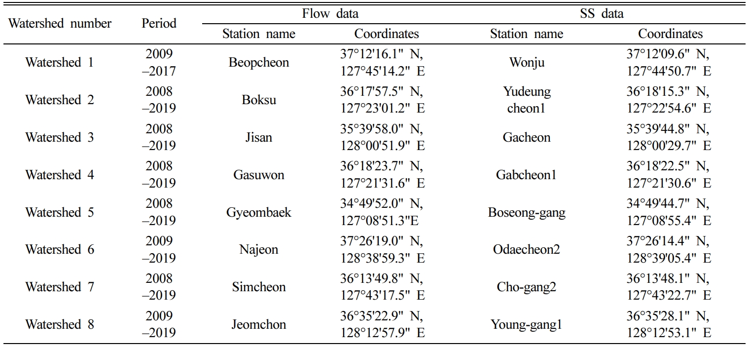
To evaluate the watershed-scale applicability of the ArcSATEEC model, the measured sediment yield data are necessary. In the study, locations at which the flow rate data and suspended solid (SS) data can be collected were selected so that the measured sediment yield could be defined (Table 1). As for the flow rate and SS data, the data from the Water Environment Information System of the National Institute of Environmental Research (http://water.nier.go.kr/) were used. Based on the period of available flow rate and SS data, the application period of the ArcSATEEC model was determined (Table 1).
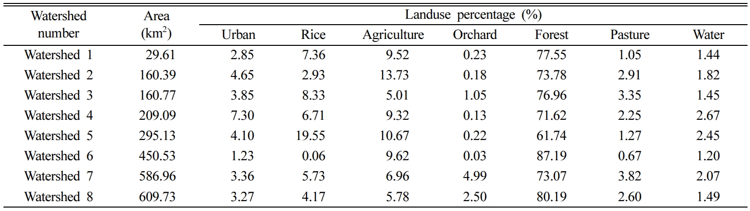
Based on the digital topographic map and the landuse map in 2007, provided by the Ministry of Land, Infrastruc-   ture and Transport and the Ministry of Environment, the watershed area ranged from 29.61 km² (Watershed 1) to 609.73 km² (Watershed 8). In terms of landuse, the forest area covered the highest proportion in all watersheds in the range from 61.74% (Watershed 5) to 87.19% (Watershed 6) (Table 2), followed by Agriculture and Rice. Orchard, pasture, and water.
 
2.2. Description of the LOADEST model for monthly sediment yield computation
To determine the estimation accuracy or correction/test results of a hydrologic model, a comparison with the measured data is required. In many cases, flow rate and water quality data can be measured at specific points in time, while the daily or monthly net loads (e.g., kg and ton) from the flow rate and pollutants are not measured. Therefore, it is necessary to process the measured flow rate and SS concentration data to define the measured monthly sediment yield (kg or ton).
The LOADEST model, the best fit regression model, can estimate pollutant loads based on the flow rate by defining the correlation between the flow rate and water quality concentration. It has nine regression equations to estimate pollutant loads, and can automatically determine a regression equation with high estimation accuracy according to the flow rate and water quality data. Moreover, its applicability has been verified from several water-quality-related studies. Oh et al. (2014) predicted weather in 18 areas in the southeastern United States using the K-nearest neighbor resampling technique and calculated the daily flow rate, and then they applied the results to the LOADEST model to estimate total daily nitrogen (T-N). Sun et al. (2013) identified the long-term trend in the pollutant loads of the nitrogen and phosphorus released from the upstream areas of the Yangtze River and Three Gorges Dam in China using the LOADEST model. Jha and Jha (2013) evaluated the applicability of the LOADEST model for the total pho-   sphorus and nitrogen observed in the Neuse River in North Carolina, USA, the estimation results for the total phosphorus and nitrogen exhibited high accuracy. The model was used to estimate monthly sediment loads in the La Sueur River watershed of 2,850 km² (Folle et al., 2007), in the Galveston and Matagorda watersheds (Onami et al., 2012). Moreover, the estimated monthly sediment yield by the LOADEST was used calibrate SWAT model(Wang et al., 2016) Major purpose of the model is to interpolate pollutant load data from intermittently measured flow and water quality concentration data, the model can be used to estimate continuous daily, monthly, and yearly pollutant loads. However, the model does not consider watershed characteristics such as landuses, soils, topography, and climates, therefore it is not available to simulate landuse or climate changes.
Hence, in this study, the monthly sediment yield was calculated based on the LOADEST model using the measured flow rate, and SS data and the results were used as the reliably estimated monthly sediment yield to correct and verify the monthly sediment yield estimated by ArcSATEEC.
 
2.3. Estimation of the monthly potential soil loss using ArcSATEEC
USLE estimates the potential soil loss (ton/ha/year) per unit area over a long time period. The USLE requires the following five factors: the rainfall erosivity factor (R factor, MJ·mm/ha·yr·hr), the soil erodibility factor (K factor, Mg·hr/MJ·mm), the slope length and slope steepness factor (LS factor, dimensionless), the crop and cover management factor (C factor, dimensionless), and the conservation practice factor (P factor, dimensionless). The R factor reflects the conditions of rainfall which leads to soil loss, while K, LS, C, and P indicate the degree of loss according to the soil attributes, the slope or slope length on soil loss, the condition of the ground surface that covers the soil and the furrow direction in agricultural lands, respectively.
 

 
where A is potential soil loss (ton/ha/year), R is the rainfall erosivity factor, K is the soil eridibility factor, LS is the slope length and slope steepness factor, C is the crop and cover management factor, and P is the conservation practice factor.
In areas where the precipitation or crop growth conditions show monthly variance, such as South Korea, the impact of monthly variations needs to be reflected when estimating potential soil loss (Park et al., 2010). They can be reflected by the R and C factors, which are related to rainfall and crop growth in USLE, respectively.
The R factor is not calculated simply using rainfall, but is defined by calculating the kinetic energy generated when raindrops fall on the ground surface. As for the calculation of kinetic energy, Whischmeier and Smith (1978) presented the method of calculating the R factor for rainfall event (Equations 2-5). For rainfall event classification, if the interval between events is less than six hours, it is defined as one single rainfall event and the minimum rainfall for the occurrence of soil loss is 12.7 mm. In addition, although the rainfall is less than 12.7 mm but is more than 6.24 mm within 15 min, the model assumes that soil loss occurred.
 

 
where I is the rainfall intensity (mm/hr), e is the kinetic energy per unit time (Kinetic energy, MJ/ha·mm), P is the rainfall per unit time (mm), E is the kinetic energy per rainfall event (MJ/ha), I_30max is the maximum 30-min rainfall intensity (mm/hr), and R is the R factor (MJ·mm/ha·hr).
To calculate the R factor using equations 2 - 5, rainfall data that can express the maximum 30-min rainfall intensity is necessary. Therefore, it is difficult to calculate the R factor for a long period of more than several years and for a number of points. Hence, Risal et al. (2016) and Kongju National University (2016) proposed equations that can calculate the monthly R factor for a total of 75 locations of the Korea Meteorological Administration (KMA) using the sum of monthly rainfall, and regression equations with different indices and coefficients depending on the area. In this study, the R factor was calculated by applying the daily rainfall data to the R factor regression equation for 47 different KMA locations from which monthly rainfall data were collected.
As the surface cover condition by crops may vary depending on the crop type and its growth condition, Kongju National University (2016) constructed a database on the monthly C factor by investigating the crop cultivation schedule for the Geumgang, Nakdonggang, Seomjingang/Yeongsangang, and Hangang watersheds, and using the SWAT model, and the database was stored in ArcSATEEC. In this study, this database was used to reflect the monthly surface cover condition for agricultural lands. These monthly R and C factors are distinct features which provide the opportunity to estimate monthly potential soil losses in ArcSATEEC (Equation 6).
 

 
where A_i is potential soil loss for month i, R_i is the rainfall erosivity factor for month i, and C_i is the crop and cover management factor for month i.
The value of the P factor is determined by the environmental conditions and management method of the cultivated land (Whischmeier and Smith, 1978), such as contouring, contour strip cropping, and up and downhill culture. To reflect these domestic conditions, Jung et al. (2004) proposed a method to calculate the P factor based on three variables (conditions, such as crop type, furrow direction, and mulch presence) for the cultivated lands in South Korea. 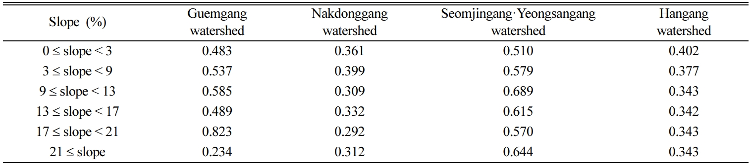The application of this method, however, can be challenging for large watersheds because investigating all cultivated lands is practically difficult even though it can be applied to small watersheds where field surveys are possible. Thus, Yu et al. (2018) conducted a field survey on the crop cultivation method and slope of each area for the representative locations of the four major river watersheds (Geumgang, Nakdonggang, Seomjingang/Yeonsangang, and Hangang watersheds)(Table 3) so that the P factor could be determined by the field slope in each watershed based on the method proposed by Jung et al. (2004).
The K factor was determined using the precision soil map provided by the Agricultural Science and Technology Institute of the Rural Development Administration, and the soil environmental map service of the Korean Soil Information System. The LS factor was estimated by the Equation 7 which is employed in ArcSATEEC, after creating DEM using the digital map provided by the National Geographic Institute (Equation 7) (Whischmeier and Smith, 1978).
 

 
where LS is the LS factor, λ is the slope projection distance (m), β is the slope (radian), and m is a slope-related variable.
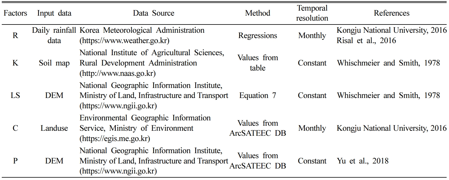
The R, K, LS, C, and P factors used in this study are given in Table 4.
 
2.4. Correction factor for potential soil loss estimation by ArcSATEEC
ArcSATEEC can reflect the monthly conditions of South Korea such as the R and C factors, but uses the same factors as USLE for estimating potential soil loss. In other words, the value estimated by ArcSATEEC does not represent the actual sediment yield (amount of the eroded soil in the watershed that reached the watershed outlet), thus it can be only compared with the sediment yield by the LOADEST after applying a correction factor, such as the sediment delivery ratio (SDR) (Wischmeier and Smith, 1965; Wischmeier and Smith, 1978; Park et al., 2007; Kim et al., 2017). SDR is defined as the ratio of the sediment yield that reached the watershed outlet to the total amount of eroded soil in the watershed; it is affected by the surface runoff, peak flow, watershed area, watershed slope, watershed geometry, rainfall type, landuse conditions, soil attributes, crop type, and growth condition. Various methods have been used to calculate SDR, including a method that considers coefficients together with the slope or area of the watershed (USDA, 1972; Vononi, 1975; Williams, 1977), a method that considers the curve number and watershed area (Williams and Berndt, 1977), a method that considers the rainfall-runoff volume (Song et al., 2019), and a method that calculates SDR for each cell of GIS data (De Rosa et al., 2016).
This indicates application of SDR allows comparison of the potential soil loss estimated using USLE or other models having an approach similar to that of USLE with the sediment yield at the watershed outlet. Different values of the correction factor can be defined differently depending on the target watershed considering environmental condition. USLE has been widely used is in soil loss estimation because it requires only five factors, and the potential soil loss can be estimated only by multiplying these factors. ArcSATEEC is an improved model of USLE by taking into account the seasonal variance while maintaining the model simplicity. In the study, in order to maintain the model simplicity when including the correction factor to convert potential soil loss into sediment yield, a straightforward approach to determine the factor was investigated.
When the monthly measured values for the sediment yield at the watershed outlet are compared with the monthly estimated values by a hydrologic model, the estimated values can be accepted when the difference between simulated and estimated values is no bigger than 45%, and the coefficient of determination (R²) is no smaller than 0.65 according to Duda et al. (2012). They can be accepted when the Nash-Sutcliffe efficiency (NSE) is 0.50 or higher according to Skaggs et al. (2012), and when the absolute error (%) is less than 50% according to Herr and Chen (2012). Wang et al. (2012) mentioned that the estimated values can be accepted when NSE is 0.50 or higher, R² is 0.60 or higher, and percent bias (PBIAS) is within ±15%. Moriasi et al. (2015) stated that the estimated values are acceptable when NSE is 0.45 or higher, R² is 0.40 or higher, and PBIAS is within ±20%. Song et al. (2019) determined the reliability of the estimated values considering the significance by the t-test when NSE was 0.4 or higher and R² was 0.5 or higher. In this study, based on these criteria, it was determined that the sediment yield could be accepted when both NSE and R² were 0.45 or higher, and the significance by the t-test was satisfied. The p-value was examined for the significance probability of 95% (signifi-   cance level α=0.05), and the estimated value was determined to be reliable when the p-value was higher than the significance level (when the test statistic was within the range of the threshold).

3.1. Comparison of monthly soil erosion by LOADEST and ArcSATEEC
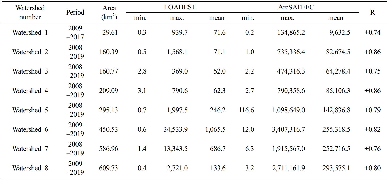
The monthly sediment yield by the LOADEST model was calculated using the daily measured flow rate and SS data (Table 5). The mean monthly sediment yield was lowest (52.0 ton/month) in Watershed 3 and highest (1,065.5 ton/month) in Watershed 6. In addition, the mean monthly sediment yield was hardly proportional to the watershed area. For example, the watershed areas of Watersheds 1 and 2 were 29.61 and 160.39 km², respectively, indicating that the area of Watershed 2 was approximately 5.4 times larger. However, the mean monthly sediment yields were 71.6 and 71.1 ton/month, respectively, exhibiting no significant difference. When comparison between Watersheds 5 and 8 showed that were the mean monthly sediment yield was higher for Watershed 5 (246.2 ton/month) than Watershed 8 (133.6 ton/month) although compared, the watershed areas were 295.13 and 609.73 km², indicating that area for Watershed 8 (609.73 km²) was approximately 2.1 times larger than Watershed 5 (295.13 km²). It was also difficult to find correlations between the minimum and maximum monthly sediment yields and the watershed area.
The mean monthly potential soil loss by ArcSATEEC showed a tendency to generally increase as the watershed area increased. For the minimum and maximum values of the monthly potential soil loss, however, correlations between them and the watershed area were difficult to find as with the minimum and maximum values of the monthly sediment yield by LOADEST. For example, while the watershed area increased from Watershed 5 to Watershed 8, the minimum value of the monthly potential soil loss rather exhibited a tendency to decrease but the maximum value increased or decreased repeatedly. In other words, it was also difficult to find a correlation between the monthly potential soil loss by ArcSATEEC and the watershed area.
When the monthly sediment yield by LOADEST was compared with the monthly potential soil loss by ArcSATEEC, the correlation coefficient (R) exceeded +0.70 for all the watersheds as it ranged from +0.74 (Watershed 1) to +0.86 (Watersheds 2 and 4) (Table 5). When the correlation coefficient between two samples is +0.70 or higher, a strong positive linear relationship is generally considered between the two samples (Ratner, 2009). Therefore, it was assumed that the monthly potential soil loss by ArcSATEEC could reflect the tendency of the sediment yield at the watershed outlet.
However, the monthly potential soil losses estimated by ArcSATEEC were significantly higher than the monthly sediment yield by LOADEST, from 135 times (Watershed 1) and up to 2,197 times (Watershed 8). This is because ArcSATEEC has the same approach as USLE when estimating the potential soil loss, and, thus, it has the limitations of USLE. In other words, the potential soil loss estimated by ArcSATEEC displayed very large values, compared to the sediment yields by LOADEST. Therefore, it was confirmed that the application of the correction factor is necessary to compare the potential soil loss by ArcSATEEC with the sediment yield at the watershed outlet.
 
3.2. Correction of monthly potential soil loss by ArcSATEEC
Although rainfalls are closely related to the sediment yield as soil loss mainly occurs during rainfall. It might be necessary to exclude the R factor in the course of defining the correction factor to avoid redundancy because it was already used for calculating the potential soil loss. DEM has information on the altitude or slope of the watershed; thus, elements for the slope and slope length can be extracted and used. Such elements, however, have already been reflected to the LS factor. In addition, soil attributes are the elements that have been reflected by the K factor. In other words, there is a need to replace or exclude one of USLE factors when extra factor is applied in the process. For instance, the R factor was replaced to the terms of runoff volume and peak runoff rate in the Modified Universal Soil Loss Equation (MUSLE)(Williams, 1975), since rainfall and runoff are similar components in soil loss estimation.
As no correlation was found between the watershed area and sediment yield for the target watersheds of this study (Table 5), using the watershed area for the definition of the correction factor is also considered to be difficult. Consequently, although the correction factor is necessary to compare the potential soil loss estimated using USLE or a similar approach with the measured value, evaluation of the correction factor is limited because it needs to maintain simplicity.
As the sediment yield showed a tendency of being linearly proportional to the potential soil loss for the target watersheds of this study, it was assumed that reasonable sediment yield can be estimated if the size of the estimated value is adjusted for each watershed. Therefore, the estimated sediment yield for month i was defined as the product of the potential soil loss_i for month i, and the correction factor (CF), an invariable number (Equation 8).

Estimated sediment yield_i = CF × Potential soil loss_i                        (Eq. 8)
 
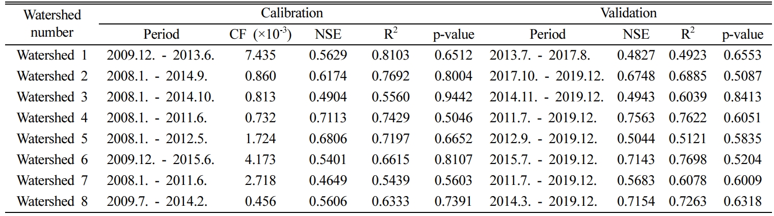
To estimate CF, the period in which the monthly potential soil loss of each watershed was estimated, was divided into calibration and validation periods. The value of CF was determined by comparing the sediment yield by the LOADEST during the calibration period with the estimated sediment yield by ArcSATEEC. During the validation period, the sediment yield by the LOADEST and estimated sediment yields were compared by applying the determined CF.
The determined CF for each watershed ranged from 0.456 × 10^-3 (Watershed 8) to 7.435 × 10^-3 (Watershed 1). NSE and R² for the sediment yield by the LOADEST and estimated sediment yields were 0.45 or higher, and the p-value also exceeded the significance level for all the watersheds, indicating that the model was well corrected by CF (Table 6). In addition, NSE and R² for the test period were 0.45 or higher and the p-values were above the significance level for all the watersheds. 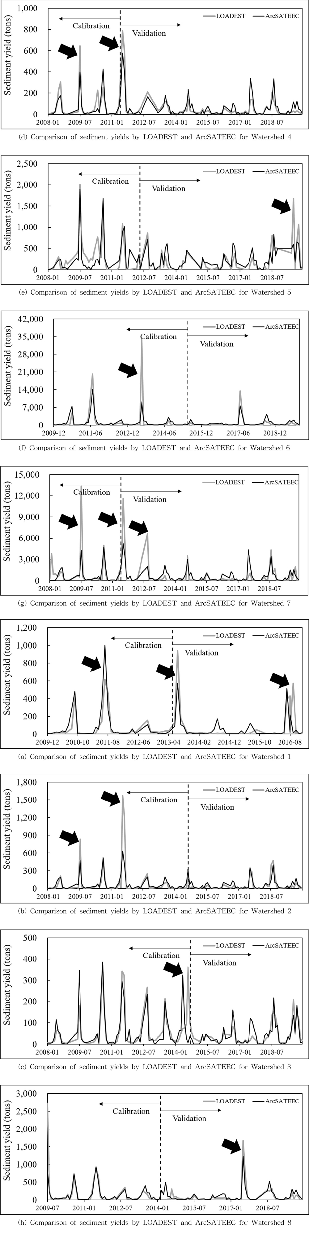Therefore, it was concluded that the test of the model was successful. Several distinct features were found in comparison of monthly sediment yields by LOADEST and ArcSATEEC. The first feature was that, the potential soil loss estimated by ArcSATEEC tended to be linearly proportional to the sediment yield that actually occurred, indicating that the ArcSATEEC model could be sufficiently corrected and tested using the correction factor in the form of an invariable number rather than a complicated correction factor with additional variables. The second feature was that the potential sol loss estimated by ArcSATEEC which has similar approach to USLE were significantly overestimated, compared to the sediment yields by LOADEST, although the tendencies of monthly potential soil loss to sediment yields were similar (Fig. 1(a) - (h)). CFs are proportions (or percentages) to represent the sediment yields reached watershed outlet, the CFs as percentages ranged from 0.046% (Watershed 8) to 0.744% (Watershed 1), The result are similar to the proportions of other USLE application for watershed. Park et al. (2014) reported that 1.12% of potential soil loss reached watershed outlet, and it was from 0.08% to 1.67% in the study of Santos et al. (2017). Therefore there is a need to correct or adjust the potential soil loss estimated by USLE and similar approaches so that they can be compared to the actual sediment yield at watershed outlet. The third feature was that watershed area does not influence sediment transportation. Comparing the CFs for Watershed 1 and 2, CFs were significantly decreased from 7.435 × 10^-3 to 0.860 × 10^-3 while the areas were increased from 26.61 km² to 160.39 km². However, CFs were increased when watershed areas were increased in the comparison of Watershed 4 and 5. Therefore, watershed area can not be used to determine or explain the proportions of sediment yield reached watershed outlet.
As it stated above, comparing the sediment yields by ArcSATEEC to the ones by LOADEST, the tendencies were similar (Fig. 1(a) - (h)), however ArcSATEEC missed the peak points of monthly sediment yields at the time steps indicated by arrows in the figure. This is because the sediment yields by LOADEST was estimated by flow rate, while ArcSATEEC estimated potential soil loss using precipitation. Therefore there is a possibility of providing differences between the estimated sediment yields by ArcSATEEC and the actual sediment yields at the time step of precipitation and flow have different behaviors. In other words, if watershed condition (e.g. irrigation and drainage, reservoirs, water uses by the inhabitant, etc.) influences the rainfall-runoff process, the differences might be observed.

The USLE has been widely used for potential soil loss estimation because the model requires only five factors (i.e. rainfall erosivity factor, soil erodibility factor, slope and slope steepness factor, crop and cover management factor, and conservation practice factor), and it is capable of calculating the potential soil loss by multiplying these five factors. However, the model only estimates the annual average values of soil loss, thus has limitations in reflecting the seasonal variances of soil losses in South Korea (Wischmeier and Smith, 1965; Wischmeier and Smith, 1978; Yu et al., 2017). ArcSATEEC was developed to overcome these limitations and calculate the monthly potential soil loss. ArcSATEEC can reflect seasonal variance while maintaining the model simplicity of USLE, but it cannot be compared with the measured value because it estimates the potential soil loss as with USLE rather than the sediment yield at the watershed outlet.
Therefore the application of the SDR is required to compare the potential soil loss with the measured sediment yield. SDR is a type of correction factor that may vary depending on the watershed. Various approaches have been used to define SDR, from the methods that used the area, slope, and curve number of the watershed to those that considered the rainfall-runoff volume or used sophisticated equations. When such SDR calculation methods are applied to USLE and similar models, it is important to maintain the model simplicity as well as to avoid elements that overlap with the factors required to calculate the potential soil loss.
In this study, ArcSATEEC was applied to eight watersheds in South Korea and examined the definition of the correction factor through a comparison with the sediment yield by the LOADEST. The monthly potential soil loss by ArcSATEEC exhibited a significant difference from the sediment yield by the LOADEST, but they tended to be linearly proportional to each other. Thus, it was confirmed that a size adjustment of the estimated value alone could exhibit reliable estimation accuracy when compared with the sediment by the LOADEST. Therefore, the possibility of estimating the sediment yield by applying an invariable number without using the watershed area, or elements that overlap with other factors that were used to calculate the potential soil loss, were examined. As both the correction and test processes of sediment yield estimation for the eight watersheds exhibited reliable results, the proposed correction factor definition method was assessed to be valid.
Based on the results of this study, it is verified that the estimated value by USLE and similar methods can overestimate the amount of the actually eroded soil because the potential soil losses significantly differs from the actual sediment yield. It was also found that the potential soil loss can be sufficiently corrected to be the estimated sediment yield using an invariable number without a complicated process if the potential soil loss has a tendency to be proportional to the sediment yield by the LOADEST.

This subject is supported by Korea Ministry of Environ-  ment as “The SS (Surface Soil conservation and manage-  ment) projects; 2019002820001”.